
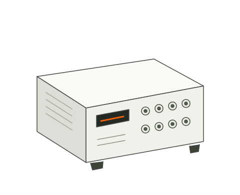
 Concept illustration↗
EQUIPMENT SERIES
T8-3X Dynamic Signal Analyzer
Acquire and analyze vibration, shock, sound pressure, dynamic force, pressure and voltage signals for measurement, structural response and modal-test workflows.
T8-3X
APPLICATION NOTE · T8-DSA-404
The channel filtering module is a signal filtering tool for vibration and acoustic testing: four filter types (band-pass, band-stop, low-pass, high-pass), adjustable order from 1 to 64 and a zero-phase algorithm with no time delay. Four views compare waveforms and spectra before and after filtering, and results export to Excel. It removes two common problems of conventional filters — shifted waveforms and hidden distortion — and serves as the preprocessing step for condition monitoring, fault diagnosis and acoustic analysis.
Example: a triangle wave on channel 1 is band-pass filtered from 100 to 250 Hz with order 16; the high-frequency content is cleanly removed, as the before-and-after waveforms and spectra show.
| Area | Name | Function |
|---|---|---|
| Left | Channel selection | Eight check boxes for the channels to filter |
| Left | Filter settings | Filter type, order (1–64), lower and upper cut-off frequencies |
| Left | Buttons | Stay on top, export all data (Excel), help, refresh |
| Top | Filter statistics | Nine columns: number, channel, filter type, order, f1, f2, RMS before and after, attenuation in dB |
| Lower right | Four views | 2 × 2: channel waveform, channel FFT spectrum, filtered waveform, filtered spectrum |
| Type | Parameters | Effect |
|---|---|---|
| Band-pass | f1 to f2 | Keeps only components between f1 and f2 |
| Band-stop | f1 to f2 | Removes the band between f1 and f2 (for example 50 Hz interference) and keeps both sides |
| Low-pass | Cut-off = f2 | Keeps components below f2 and removes high-frequency noise |
| High-pass | Cut-off = f1 | Keeps components above f1 and removes DC and low-frequency drift |
Bearing and gearbox fault signatures are often buried in strong background noise. Band-pass filtering first extracts the diagnostic band, for example around a bearing outer-race frequency; envelope demodulation and zoom analysis then give more reliable conclusions.
50 Hz supply interference and its harmonics are the most common contamination in field tests. A band-stop filter removes 50 Hz precisely (f1 = 48, f2 = 52) and keeps all other content. Because the algorithm is zero-phase, the waveform does not shift in time and events can still be located exactly.
Band-pass filtering isolates one resonance band so that its time response, such as beating or decaying oscillation, can be observed, supporting modal analysis and resonance investigation.
Separate the band of interest, for example 500 Hz to 4 kHz for speech interference, together with the acoustic functions (frequency weighting, octave analysis, sound quality).
The four views show the effect of each parameter immediately and explain cut-off frequency and filter order clearly.
Filter delay and phase response depend on the design:
The source describes a real, non-negative, even-symmetric mask applied to a complete FFT frame:
A real, non-negative, even mask adds no phase shift to retained frequency components. Whole-frame filtering nevertheless has finite-record boundary effects and can change peaks and waveform shape. It is not generally equivalent to forward-backward filtering: applying a filter twice changes its magnitude response as well as its phase. Inspect the frame boundaries and validate timing for the measurement task.
The mask magnitude follows the maximally flat Butterworth response, −3 dB at the cut-off frequency fc:
Low-pass: |H(f)| = 1 / √(1 + (f / fc)^(2N)) High-pass: |H(f)| = 1 / √(1 + (fc / f)^(2N))
N is the filter order (1–64). The stop-band slope is 6N dB per octave; order 10 gives 60 dB per octave.
| Type | Mask construction |
|---|---|
| Band-pass | H = high-pass(f1) × low-pass(f2) |
| Band-stop | H = 1 − (1 − low-pass(f1)) × (1 − high-pass(f2)) |
| Low-pass | H = low-pass(f2) |
| High-pass | H = high-pass(f1) |
Exponents are computed in logarithmic space with upper and lower limits (values beyond them are set to 0 or 1), so no order or frequency ratio causes overflow.
The supplied manual reports the following NumPy examples. The test code, inputs and T8 software implementation were not independently validated for this website; these values are illustrative source results, not Vectalen verification evidence:
| Check | Result |
|---|---|
| FFT round-trip identity error | 3.5 × 10⁻¹⁰ |
| In-band gain (500 Hz, band-pass 100–1000 Hz) | 0.998 |
| Stop-band residual, order 4 | 0.062 (about −24 dB, consistent with theory for order 4) |
| Stop-band residual, order 64 | 2 × 10⁻¹⁸ (close to an ideal brick wall) |
| Cross-correlation delay | lag = 0 (exactly zero delay) |
| Item | Conventional point-by-point IIR/FIR filtering | T8 channel filtering |
|---|---|---|
| Time delay | Depends on design and processing method | None |
| Phase distortion | Depends on phase response; linear-phase FIR is possible | None |
| Locating impact events | Timing interpretation depends on the filter delay | No added phase shift from the stated mask; check finite-record effects |
| Checking the filter effect | Depends on the software | Four views on one screen |
| Filter order | Depends on numerical implementation | Source-specified orders 1–64; validate the selected response |
| Quantified effect | None | RMS before and after and attenuation in dB |
| Data delivery | Depends on the software | Excel export of parameters and spectra |
Open channel filtering from the main menu (or the corresponding extended analysis menu). The window loads the current frame and draws it.
| Application | Type | Order | Cut-off |
|---|---|---|---|
| Remove 50 Hz supply interference | Band-stop | 32–64 | f1 = 48, f2 = 52 |
| Noise reduction before bearing diagnosis | Band-pass | 4–10 | Characteristic frequency ±30 % |
| Remove drift from acceleration signals | High-pass | 4–8 | f1 = 1–10 |
| Post-acquisition high-frequency filtering | Low-pass | 8–16 | f2 below one quarter of the sampling rate |
| Isolate a structural resonance band | Band-pass | 8–16 | Resonance peak ±20 % |
| Question | Answer |
|---|---|
| Why do both ends of the filtered waveform show a few milliseconds of transition? | This is normal. Whole-frame frequency-domain filtering assumes a periodic extension of the signal, so the frame edges have a boundary effect. Exclude about 2–5 periods of the lowest frequency at each end; steady signal sections are not affected. |
| Is a higher order always better? | No. A higher order gives steeper edges but stronger ripple in the pass band near the cut-off (Gibbs effect). Choose the order that separates the target components; 4–16 is usually enough. |
| Why does the lower cut-off field do nothing in low-pass mode? | Low-pass uses only f2 (f1 shows “-”), and high-pass uses only f1. Band-pass and band-stop use both. |
| Does filtering change the original data? | No. Filtering runs inside the window; the original data arrays, the main display and the stored data are not changed. |
| How should a negative or 0 dB attenuation be read? | Attenuation = 20 · lg(RMS after / RMS before). When band-pass or high-pass filtering removes the band that carries most of the energy, the value is strongly negative; when the removed band carries little energy, it is close to 0. Check that the value is reasonable for the application. |
| Item | Specification |
|---|---|
| Channels | 8, freely selectable |
| Filter types | Band-pass, band-stop, low-pass, high-pass |
| Order | 1–64 (stop-band slope 6N dB per octave) |
| Algorithm | Real symmetric mask in the FFT domain; zero phase, no time delay |
| Magnitude response | Butterworth maximally flat; −3 dB at the cut-off |
| Display | Four views (2 × 2), double-click to maximize, refreshed every frame |
| Statistics | RMS before and after, attenuation in dB, per channel |
| Data export | Excel (filter parameters and complete spectra) |
| Interface language | Chinese, English or Russian |
YOUR NEXT STEP
Choose a family or describe your application. Prepare one inquiry with the details that matter.
Prepare your inquiry